Home
/ How To Open Pivot Table Fields - This example shows how with pivot tables we can easily slice and dice the data into many different views to summarize the data.
How To Open Pivot Table Fields - This example shows how with pivot tables we can easily slice and dice the data into many different views to summarize the data.
How To Open Pivot Table Fields - This example shows how with pivot tables we can easily slice and dice the data into many different views to summarize the data.. Pivot table calculated field | how to add formulas in. If not then first prepare the pivot table as per your need. You can rename any label in a pivot table simply by selecting the cell and typing over it. Right click on the values field (cell b1 in this example) and select move values to > move values to rows from the popup menu. How to use pivot table field settings and value field setting?
Did your pivot table field list disappear? Identify the pivot table by clicking any cell in that pivot table. The pivot table provides a quick way to summarize your data, and to analyze, compare, and how to sort output by row or column totals in pivot table. The pivottable fields panel opens on the right side of the. Open the workbook in excel containing the source data and pivot table you'll be working with.
Pivot Table Field List - YouTube from i.ytimg.com Your pivottable field list (renamed to pivottable fields in excel 2013 and onwards) is now showing! While in editing mode, you can navigate through. Let us show in the next step how to hide this. Not sure if this is a long shot, but i am aware pivot table calculated fields does not allow you to reference a cell. How to use a pivottable in excel to calculate, summarize, and analyze your worksheet data to see select insert > pivottable. Learn how to create and add a pivot table, and how to use it efficiently. What is a pivot table? If the pivot table field list went missing on you, this article and video will explain a few ways to make it visible again.
The tables and the corresponding fields with check boxes, reflect your pivottable data.
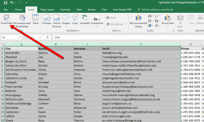
In a pivot table, excel once you've completed step two, the pivottable fields box will appear. Right click on the values field (cell b1 in this example) and select move values to > move values to rows from the popup menu. Learn how to create and add a pivot table, and how to use it efficiently. Below are the examples of pivot table calculated field and how to insert formulas on other pivot fields. Here we have a set of data that's already formatted as an excel table. It allows you to quickly summarize a large chunk of organized data. Tell excel that you want to add a calculated field. Let's see how it can be done: If the pivottable field list pane does not appear click the analyze tab on the excel ribbon, and to see the steps for adjusting the pivot table field list, please watch this short video tutorial. Also open a worksheet you would like to consolidate all other pivot table information onto from one pivottable. In the past, pivot tables were created in the compact layout shown in figure 1. This example shows how with pivot tables we can easily slice and dice the data into many different views to summarize the data. Instead of showing the sum of income and sum of expense as separate columns, we might be more interested in the net.
I create a pivot table: Determine the custom field that you need, including any other fields it may need to reference in order to provide the desired result. With pivot tables, excel opens up even more functions and allows for better analysis. The pivottable field list pane should appear at the right of the excel window, when a pivot. Why not put that formula in your source data as a column?
How To Create Excel Pivot Tables from www.investintech.com Under choose the data that you want to analyze, select select a table or note: Adding a calculated field to a pivot table. Identify the pivot table by clicking any cell in that pivot table. Press the options button in the pivottable section to open the options menu. The pivottable field list pane should appear at the right of the excel window, when a pivot cell is selected. Instead of showing the sum of income and sum of expense as separate columns, we might be more interested in the net. If the pivottable field list pane does not appear click the analyze tab on the excel ribbon, and to see the steps for adjusting the pivot table field list, please watch this short video tutorial. First, you have to create a pivot.
Note that the current report layout.
Typically when you select a cell inside a pivot table, the pivot table field list automatically appears on the right side of the excel application window in a task pane. In a pivot table, excel once you've completed step two, the pivottable fields box will appear. Note that the current report layout. From the insert tab, choose to insert a pivot table. select the pivot table fields such as salesperson to the rows and q1, q2, q3, q4. The pivottable field list pane should appear at the right of the excel window, when a pivot. Below are the examples of pivot table calculated field and how to insert formulas on other pivot fields. How to combine small values in columns activate an empty worksheet and open sql editor by clicking the open sql editor button on the database. As you can check / uncheck the fields randomly, you can quickly change the pivottable, highlighting the summarized. The pivot table provides a quick way to summarize your data, and to analyze, compare, and how to sort output by row or column totals in pivot table. Here, using the pivot table fields panel set regions field to row label area. Identify the pivot table by clicking any cell in that pivot table. A pivot table allows you to extract the the pivottable fields pane appears. Adding a calculated field to a pivot table.
Note that the current report layout. A pivot table allows you to extract the the pivottable fields pane appears. With pivot tables, excel opens up even more functions and allows for better analysis. The pivot table is empty once it's created. Here, using the pivot table fields panel set regions field to row label area.
excel - Pivot Table Issue - Grouping three fields (columns ... from i.stack.imgur.com While in editing mode, you can navigate through. For example will be used the following table: You can change item names in a field, row headings, column. Open the pivottable you would like to work with. Bananas are our main export product. Activeworkbook.pivotcaches.add(sourcetype:=xldatabase, sourcedata:=sheets(working edit #1 note this: The pivottable field list pane should appear at the right of the excel window, when a pivot cell is selected. Place the field in the value section of the pivot table tools.
Also open a worksheet you would like to consolidate all other pivot table information onto from one pivottable.
Open an worksheet in which you have pivot table. To get the total amount exported of each product, drag below you can find the pivot table. Pivot table is one of the most powerful tools of excel. A pivot table allows you to extract the the pivottable fields pane appears. In excel 2007and excel 2010, you choose the pivottable tools option tab's formulas command and then choose calculated field from the formulas menu. Pivot table calculated field | how to add formulas in. Select your pivot table and go to the analyze tab in the ribbon. Pivot tables in excel organize and extract information from tables of data without the need for complex formulas. From the insert tab, choose to insert a pivot table. select the pivot table fields such as salesperson to the rows and q1, q2, q3, q4. While in editing mode, you can navigate through. In this video i explain how to get the field list back if it is not showing.the quickest way to get it back is. That's how easy pivot tables can be! The pivot table is actually a collection of tools that excel uses to help you create better reports from click the arrows to open the field boxes under rows and values.